Repeat this construction recursively on each of the two new squares. The figures below show the next two iterations.
 |
 |
|
| Iteration 2 | Iteration 3 |
The limit of this construction is called the Pythagorean Tree (or Pythagoras Tree).
For the first function, corresponding to the upper left square, we must scale by \(\cos(\alpha)\) and rotate counterclockwise by \(\alpha,\) then translate straight up. For the second function, corresponding to the upper right square, we must scale by \(\sin(\alpha)\) and rotate clockwise by 90°−\(\alpha\), then translate the point at the origin to the point at the right angle in the triangle. Finally, the third function is just the identity. This keeps the squares already drawn in their current locations while the first two functions add additional squares.
|
\({f_1}({\mathbf{x}}) = \left[ {\begin{array}{*{20}{c}}
{{{\cos }^2}(\alpha )} & { - \cos (\alpha )\sin (\alpha )} \\
{\cos (\alpha )\sin (\alpha )} & {{{\cos }^2}(\alpha )} \\
\end{array} } \right]{\mathbf{x}} + \left[ {\begin{array}{*{20}{c}}
0 \\
1 \\
\end{array} } \right]\)
\({f_1}({\mathbf{x}}) = \left[ {\begin{array}{*{20}{c}} {{{\sin }^2}(\alpha )} & {\cos (\alpha )\sin (\alpha )} \\ { - \cos (\alpha )\sin (\alpha )} & {{{\sin }^2}(\alpha )} \\ \end{array} } \right]{\mathbf{x}} + \left[ {\begin{array}{*{20}{c}} {{{\cos }^2}(\alpha )} \\ {1 + \cos (\alpha )\sin (\alpha )} \\ \end{array} } \right]\) \({f_3}({\bf{x}}) = \left[ {\begin{array}{*{20}{c}} { 1} & {0} \\ { 0} & { 1} \\ \end{array}} \right]{\bf{x}} \) |
Note that function 3 in this iterated function system is not a contractive mapping. Therefore the theory of contractive iterated function systems cannot necessarily be applied here. However, in this case the iterates of the initial square under this iterated function system do converge to a limit set [Proof]. In fact, the iterates will converge to a limit set starting with any initial set even with the non-contractive identity map as part of the IFS [Proof]. Unlike other examples on this website, though, the limit set will depend on the initial set that is used. The image on the left below shows 10 iterations starting with a square, with \(\alpha\) = 45°. The image on the right shows 10 iterations starting with a vertical line segment.
Notice that while the "trunk" of the two trees are different, the "outer leaves" of the trees do appear to be very similar. This is because if you delete the third function from the iterated function system, the remaining two functions are contractive and thus do have a unique attractor no matter what initial set you start with. See how this works in the animation below by clicking the Play button.
In fact, functions 1 and 2 are essentially the same functions as for the Lévy Dragon, just with translation vectors shifting an additional 1 unit vertically.
Suppose you number the squares as in the figure below. The initial square is labeled with index 1. If a square has label n and a right isosceles triangle is placed on top on which two new squares are constructed, then the new square on the left will have index 2n and the new square on the right will have index 2n+1. Notice in the figure that the red squares have an even index and the blue squares have an odd index. The figure only shows the first 4 iterations. After that the squares will begin to overlap but the indexing algorithm will still apply as more iterations are done. Once a square is given a particular index, it will never change while additional squares are created.
You can now use binary notation to locate any particular square in the Pythagorean tree. For example, where would square 45 be located? Since 45 = 32+8+4+1, it would be written in binary as 101101. The left most digit will always be 1 and corresponds to the base (initial) square. For the remaining digits, a 0 means a turn to the left (red square) while 1 means a turn to the right (blue square). So to get to square 45, go left, right, right, left, right. This is illustrated in the next figure.
Where is square 116? Since 116 = 64+32+16+4, in binary this would be 1110100. So starting at the base, turn right, right, left, right, left, left (which means we need at least 6 iterations to see square 116). See below.
What about square 98156? In binary this is 10111111101101100 which has 17 digits. You would need to take 16 iterations to get to this square. This square would have been reduced by a factor of \((\sqrt{2}/2)^{16}\) = 1/256 so might be a bit too small to see on the computer screen!
The figure on the left below shows the squares with indices 1, 2, 4, 8, ..., i.e. the powers of 2. These squares form a logarithmic spiral that converge to a point (more precisely, comparable points on each square lie on a curve that is a logarithmic spiral; the figure on the right shows the curve through the corner points.) But there is really nothing special about starting with the initial square. If you start with any square in the Pythagorean tree and follow the squares off that one that always go either to the left or always go to the right, then those squares will also follow the path of a logarithmic spiral. Thus the Pythagorean tree is full of infinitely many spirals [More Details].
[Enlarge]
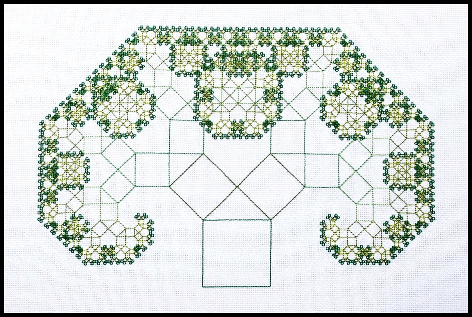
Back Stitch Design (done with IFS Construction Kit)
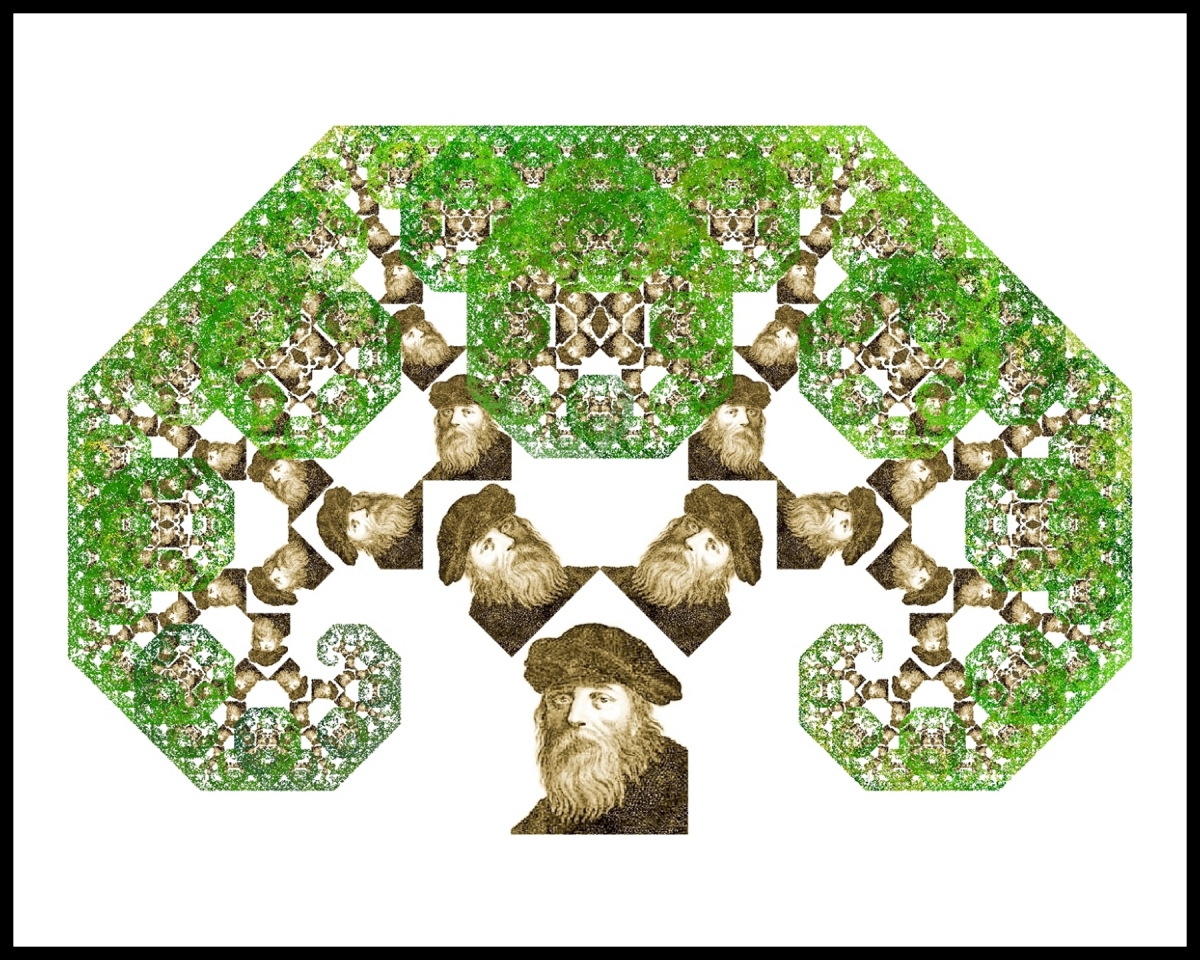
The traditional Pythagorean tree is constructed by starting with a square and constructing two smaller squares such that the corners of the squares coincide pairwise (thus enclosing a right triangle), then iterating the construction on each of the two smaller squares. When viewed as an iterated function system, however, one can start the iteration with any initial set as in the following image.
For this image I began with a common picture of Pythagoras as the initial set. The trunk of the three was constructed using 10 iterations of a slight modification of the iterated function system where the first function includes a horizontal reflection across a vertical line. This gives a reflective symmetry to the trunk by having the images of Pythagoras looking towards each other. The picture of Pythagoras was scaled and placed in just the right spot (after some experimentation) so that at each iteration the base of the new pictures will just touch at a 45° angle. The leaves of the tree consist of 500,000 points plotted using a random chaos game algorithm and colored based on Michael Barnsley's color stealing algorithm. To give the leaves a more realistic shading, the colors were stolen from a digital photograph of a field of green and yellow grass.
Constructing a Pythagorean tree with paper and scissors is a nice project for students or math clubs. Teachers can have students make a tree to display in the classroom or other public venue. Here is a picture of the first three steps of a 45-45-90 tree constructed by Kim Matthews, a math teacher in Gwinnett County, Georgia.
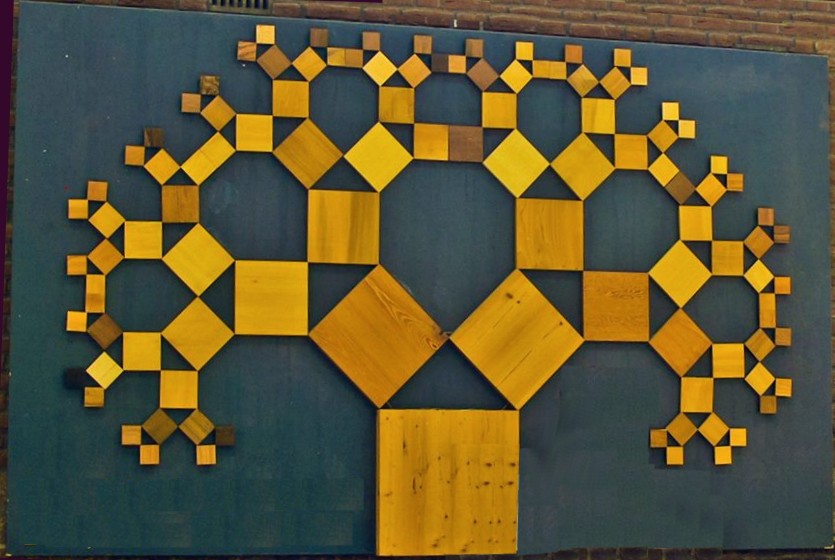
The 2013 Symmetry Festival in Delft, Netherlands, exhibited a 45° Pythagorean Tree constructed from wooden blocks.